A combinatorial problem (puzzle) is one in which various elements (pieces) can be combined (assembled) many different ways, only a few of which are the desired result (solution). The success or lack of it for any attempt at solution may not become apparent until most of the pieces are in place. For a geometrical puzzle, ideally all pieces are dissimilar and non-symmetrical, thus resulting in the maximum number of combinations for a given number of pieces. Maximum difficulty is achieved when only one correct combination exists. Since puzzles of this type can usually be made more difficult simply by increasing the number of pieces, the challenge facing the puzzle designer is to cleverly devise simple puzzles of this sort having few pieces while yet being intriguing and puzzling. In this chapter, we will introduce the subject by considering some simple two-dimensional combinatorial puzzles.
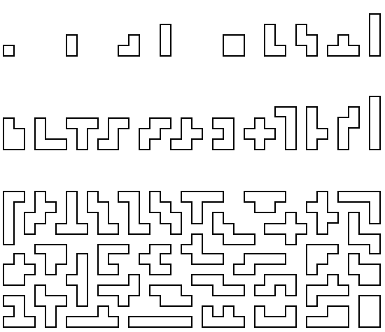
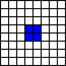
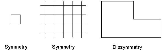
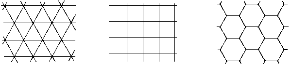
The basic building block of a geometrical combinatorial puzzle is typically a regular polygon, although other shapes or combinations of shapes are certainly possible. Whatever shape or shapes are used, the idea is to create a set of dissimilar puzzle pieces that fit together a great many different ways. Among regular polygons, the only ones that tile the plane are the triangle, square, and hexagon (Fig. 23).
Fig. 23
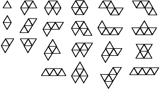
Fig. 24 illustrates all the different ways of joining triangles through size-six. Note that mirror images are not counted as separate pieces, since it is assumed these are real physical pieces that can be flipped over. These pieces are sometimes referred to as polyiamonds. The numbers of pieces are summarized in Table 1.
Fig. 24
Table 1
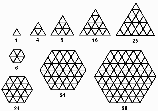
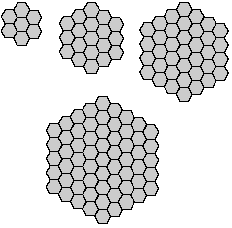
The next step is to consider what simple geometrical shapes these pieces might be assembled into. For the triangle, the most obvious patterns are triangular and hexagonal. These are shown in Fig. 25 in increasing size.
Fig. 25
Comparing the numbers in Table 1 with the total numbers of blocks in different-sized sets, we note that none of them match. At this point there are two different schools of thought. Those whose interest is primarily mathematical analysis like to work with complete sets of things, so they would probably either tinker with the definitions of the sets in an attempt to make the numbers match or perhaps abandon this particular line of inquiry. From the practical point of view, on the other hand, there is no good reason why the pieces of a puzzle must comprise a complete mathematical set in order to be interesting. The tabulation of complete sets is useful in that it shows all the pieces that are available without duplication. Example: select a set of nine six-block pieces that assembles into a size-54 hexagon. Second problem: does such a set exist having a unique solution? (Answer unknown).
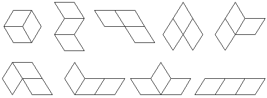
For those who do insist on working with "complete" mathematical sets, not that of the 12 pieces of size-six, nine of them can be made by joining three two-block rhombuses together all possible ways, as shown in Fig. 26. Of course, this also has practical woodworking significance. Assemble these nine pieces into a 54-block hexagon.
Fig. 26
Now see if the same can be done with another set of nine pieces coincidentally formed by joining two three-block trapezoids all possible ways.
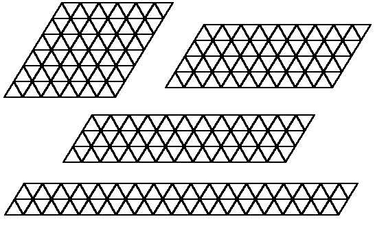
Note also that the entire set of twelve size-six pieces might be assemblable into a 72-block rhombus or rhomboid many different ways. Which of those shown in Fig. 27 are possible to assemble?
Fig. 27
For more information on amusements of this sort, see Martin Gardner's Sixth Book of Mathematical Games from Scientific American.
Continuing in the same vein, we now consider squares as building blocks (Fig. 28), with the number of pieces summarized in Table 2.
Fig. 28
Table 2
When we compare this summary with that for the triangle, the much greater versatility of the square as a combinatorial building block is apparent. The various pieces are popularly referred to as polyominoes after a book on the subject with that title by Solomon Golomb. The various sets of pieces have been the object of much investigation by mathematical analysis. Note that much of this analysis is concerned with proving mathematically where such pieces will or will not fit, which may or may not have much relevance to the design of practical geometrical puzzles.
Incidentally, the listing in Table 2 and others like it have been calculated for pieces of much larger size, often using a computer. Such pieces have little practical value in dissection puzzles beyond a certain size, the elegant simplicity of discrete dissection becomes obscured by complexity, going against the natural human inclination to reduce all things to their simplest and most functional common denominator. In combinatorial recreations of this sort, those that achieve their intended object using the fewer and simpler pieces are nearly always the more satisfactory.
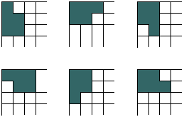
The most obvious constructions for polyomino puzzle pieces are square or rectangular assemblies. If complete sets are being considered, then Table 2 suggests that only the size-four and size-five sets look interesting. First we will dispose of the size-four set. If the reader will mark and cut the five size-four pieces out of cardboard, it should be easy to convince oneself that it is impossible to assemble them into a 4 x 5 rectangle. But how can you be sure? This problem will be used as a simple example to illustrate two common analytical approaches to puzzles of this type.
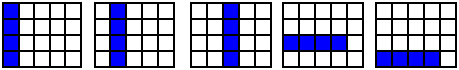
Mark a 4 x 5 board on paper. Start with the straight piece and note that there are 13 different positions it can occupy on the board. But because of symmetries, only five are distinctly different. Of these five (shown in Fig. 29), three can immediately be eliminated by inspection. The remaining two can be analyzed by placing a second piece, the square, in all possible positions and seeing what problems then arise. When one uses this method, a judicious choice of the first piece may save many steps. Usually a symmetrical piece is the best choice because there are fewer distinctly different ways that it can be placed.
Fig. 29
An alternate technique frequently used for analyzing problems of this sort is the following: Note that if the 4x5 board is checkered, it will always have 10 light and 10 dark squares. Now checker the pieces and note that four of them will always have two light and two dark squares, but the fifth will always have three of one color and one of the other (Fig. 30). Consequently, they will never fit onto the board.
Fig. 30
As already shown, joining five squares together all possible ways produces a set of 12 puzzle pieces. Popularly known as pentominoes (Fig. 31). These occupy much of Golomb's book and have received much attention from others also. The total of 60 blocks is a most fortuitous number because it has so many factors. The earliest reference to a puzzle of this sort appears to be in The Canterbury Puzzles, by Henry Dudeney, published in 1907. The idea is so obvious that it may have to many persons independently.
Fig. 31
The pentominoes are capable of being assembled into four different rectangles - 3 x 20, 4 x 15, 5 x 12, and 6 x 10. The first investigation of these by computer was probably by Dana Scott in 1958. The results were summarized in an article by C. J. Bouwkamp in the Journal of Combinatorial Theory in 1969. There are 2, 368, 1,010, and 2,339 solutions to these four rectangular assemblies. One of each is illustrated in Fig. 32.
|
| 3 x 20 - 2 Solutions |
|---|
|
| 4 x 15 - 368 Solutions |
 |
| 5 x 12 - 1,010 Solutions |
 |
| 6 x 10 - 2,339 Solutions |
Fig. 32
With 2,339 solutions, you might expect that placing the 12 pieces onto a 6 x 10 tray should be quite easy. If so, you are due for a surprise! One of the charms of puzzles of this sort is that the first few pieces fall into place and nestle together as though they were made just for each other's company. The next few pieces maybe a bit more troublesome, but they finally settle down happily into place too. It is always the last one or two pieces that are the rascals. As you carefully rearrange things to suit them, then other pieces become the outcasts. Reluctantly you have no choice but to break up combinations that seemed so content together. Alas, you have made the situation worse instead of better, for now there are three that won't go in. In a moment of frustration, you are tempted to brusquely dump the lot out of the tray and start afresh. But no, you take the gentler and wiser approach of patiently switching just a few pieces back and forth, when suddenly the solution reveals itself as the remaining empty space just happens to match the last piece. As it drops snugly into place, there is a sense of resolution and harmony that any sensible person must welcome these days, especially if you have just scanned the headlines of the daily news or perhaps driven through Harvard Square in rush-hour traffic!
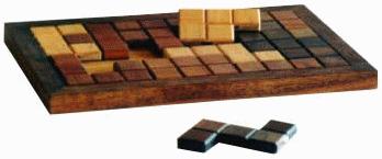
Although it was mentioned earlier that crude models will usually suffice for experimental work, that was not necessarily intended as a recommendation. Here is a case where one might well develop a deeper relationship with this captivating set of puzzle pieces by making them accurately and solidly of attractive hardwood, with a smooth finish and close fit and with a matching tray (Fig. 33). They will repay your consideration many times over.
Fig. 33
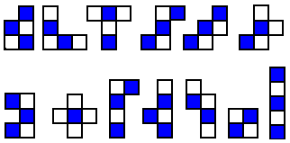
What may at first seem like a random process of placing the first few pieces on the tray is anything but. Never underestimate the amazing power of the human brain. Which gets even better with practice. For example, you will find some pieces much more cooperative than others. Piece no. 1 is the most tractable. Resist the temptation to place it early - it is your trump and should be kept in reserve until you really need it. Pieces that decline to fit nicely into the corners are the most troublesome. Piece no. 8 is the worst - it refuses altogether. Yet even it has a companion in piece no. 7, so let the pair of them mate. Try to fill the corners first, the ends next, and work toward the center.
For an even more methodical (but less entertaining) approach, consider how a complete analysis of this puzzle might be made. Number the spaces on the 6 x 10 tray 1 to 60 as shown (Fig. 34). Always try to fill the lowest numbered unfilled space with the lowest numbered remaining piece. So, start by placing piece no. 1 on space no. 1. Since this piece has no symmetry, it can be oriented four different ways by rotation plus four more when flipped over, six of which will cover space no. 1. With piece no. 1 in place, try placing piece no. 2 in the next numbered empty space. Piece no. 2 has four orientations by rotation, but because of symmetry it need not be flipped over (likewise pieces no. 3, no. 5, and no. 7). Continue placing pieces in this manner. Note that piece no. 4 has twofold rotational symmetry, so it has only two orientations plus two more when flipped. Piece no. 12 has both rotational and reflexive symmetry, so only two possible orientations. Piece no. 8 is the most symmetrical of all, with only one possible orientation. Furthermore, because of symmetries of the tray, the location of the starting piece can be confined to one quadrant.
 |
|
Fig. 34
Continuing methodically in this manner, one arrives at either a solution or an impasse. When an impasse is reached, the last piece placed is tried in every possible orientation. If that fails, the same is tried with the previously placed piece. Without belaboring all of the details, the point is that by proceeding methodically along these lines, or by some other similar scheme, one eventually tries every piece in every possible location and orientation, and compiles a complete list of solutions (or proves that none exists). If all of this sounds exceedingly arduous, it is indeed, and in the case of this particular example so much so as to be beyond practical human capability. This is where computers come into play. They are perfectly suited for this sort of mindless task. They do in seconds what might take a person days or months, and do so with much less likelihood of error.
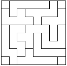
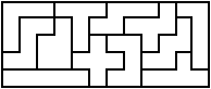
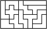
The joined-square combinatorial puzzles just described bear a close resemblance to the checkerboard dissections discussed in the previous chapter. The distinction between dissection and combinatorial puzzles has little to do with appearance, but rather with method of creation. The classification is not always precise, and the two categories tend to overlap. Consider the checkerboard puzzle shown in Fig 35, which appeared in The Canterbury Puzzles. The pieces are printed on one side only so may not be flipped.
Fig. 35
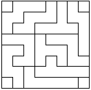
At first glance, this might appear to be just another checkerboard dissection like those mentioned in the previous chapter. Upon closer scrutiny. However, it is obvious that the pieces were not created by a process of dissection. Rather, Dudeney must have taken the set of 12 pentominoes, added the 2 x 2 square to bring the square count up to 64, assembled all of the pieces into an 8 x 8 square, and lastly added the checkering.
In trying to solve this puzzle, one might start by assuming that Dudeney probably placed the square piece symmetrically in the center for aesthetic reasons. (Before checkering, there are 65 solutions with this arrangement.) With the 2 x 2 checkered square thus centered, by placing the cross piece in each of its four possible locations, one discovers the impossibility of any such solution. This puzzle is known to have four solutions, but all with the square piece off center. Did Dudeney introduce this slight aesthetic anomaly just to confuse us? We will never know for sure but if he did, why then would he have chosen a version with four solutions instead of just one, making it that much easier? A puzzle within a puzzle!
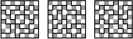
Of all the checkerboard puzzles in Slocum's Compendium, only one is said to be of recent vintage. It may appear at first glance to be just a variation of the Dudeney puzzle. But it was designed by Kathy Jones, which should alert any puzzle connoisseur to expect something thoughtfully conceived and executed. The pieces are checkered on both sides and may or may not be the same on both sides. The puzzle has 1,294 checkered solutions, and the 2 x 2 square can be in any possible position. It also solves several other problems. Three of the solutions with the 2 x 2 square in two different locations are shown in Fig. 36. Note that not quite enough information is given here to determine the exact checkering on both sides of all pieces. The puzzle is produced by Kadon Enterprises, Inc.
Fig. 36
Solving or attempting to solve a mechanically manipulative puzzle analytically, with all of the action taking place unseen inside a computer, may not sound like much fun except for the computer fanatic. Be that as it may, the computer is now frequently being used as an aid in the design and optimization of combinatorial puzzles. Many examples will be given in this book. One of the more impressive of these is the Cornucopia Puzzle.
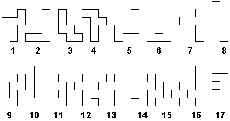
It was shown previously that joining six squares all possible ways produces a set of 35 puzzle pieces. Now, from this set, eliminate all pieces having reflexive or rotational symmetry and all those containing a 2 x 2 square because they are less desirable for various reasons already explained. The remaining 17 pieces are the set of Cornucopia pieces (Fig. 37).
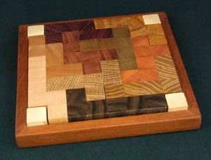
Fig. 37
A subset of any 10 of these pieces will fit onto an 8 x 8 board leaving four empty squares. There are 10 different ways that these four empty squares can be arranged in fourfold symmetry (disregarding reflections) as shown in Fig. 38.
Fig. 38
A subset of 10 Cornucopia pieces can also be assembled to form a solid 6 x 10, 5 x 2, or 4 x 15 rectangle. (Note: the 3 x 20 rectangle is impossible Can the reader discover a neat and simple proof of this? Hint: place piece no. 1, 3, 4, 5, 7, 9, 12, 13, or 15 anywhere in the 3 x 20 rectangle as in Fig. 39 and see what problem then arises.) (Answer)
Fig. 39
Combinatorial theory shows that a subset of 10 pieces can be chosen from a set of 17 pieces 19,448 different ways. Which of these subsets will fit any of the boards shown in Fig. 38, and in how many different ways? Expert puzzle analyst Mike Beeler decided to find the answers to these questions with the aid of a computer. Even with state-of-the-art equipment and clever short cuts, this probably invoked more computation than any previous puzzle analysis and by a wide margin. The final results show 8,203 usable subsets and 105,902 solutions, any one of which constitutes an interesting and challenging puzzle problem, hence the name Cornucopia. This suggested the possibility of producing a series of Cornucopia puzzles whereby each set of pieces would be unique, and each with its own unique solution or solutions. (The idea itself is also believed to be unique!). One hundred such sets were produced in wood in 1985 and are now in the hands of puzzle collectors. The remainder are contained in a stack of papers a foot high!
At the beginning of the Cornucopia project, as the computer started to spew out solutions, we wondered if any subset would be found that made all 13 patterns. Preliminary results indicated this to be very unlikely. To our surprise, however, near the end of the run one prolific subset was discovered that failed to do so by the narrowest margin. It is shown in Fig. 40, with a tabulation of all its copious solutions given in Table 3. To gain some appreciation of the power and speed of a computer, the reader is invited to make this subset of pieces and try to solve just one of the other 56 solutions listed. Now imagine all 57 of them being solved in a few seconds!
Fig. 40 - The Copious Cornucopia
| Pattern | Total Number of Solutions |
|---|---|
| A | 7 (One Shown) |
| B | 1 |
| C | 0 |
| D | 1 |
| E | 11 |
| F | 1 |
| G | 1 |
| H | 1 |
| I | 4 |
| J | 1 |
| 6 X 10 | 15 |
| 5 X 12 | 12 |
| 4 X 15 | 2 |
Table 3
With polyomino-type puzzles like Cornucopia, when many solutions are known, here is an interesting exercise: display all of them together and have several friends judge which they consider to be the most and least pleasing to the eye. If there is any consistency in the judging, try to determine what characteristics are common to those judged most or least pleasing. Finally, try to define these characteristics mathematically.
After staring at thousands of Cornucopia solutions, the author has selected the two shown in Fig. 41 as being a good pair for illustrating this game. Everyone polled by the author preferred the same one. The other one has at least four easily recognizable and describable flaws. What are they? (Answer) Paradoxically, perhaps the most distinguishing feature of a pleasing polyomino pattern is its lack of any distinguishing features! Evidently the mind's eye prefers randomness in such designs. We all know what randomness is, or think we know until we try to define it mathematically. Randomness is, almost by definition, something that cannot be defined mathematically! And even if the rules for randomness could be stated mathematically, what about the rules for the rules?
Fig. 41
To further compound this strange paradox, at the same time the eye goes to the opposite extreme and automatically takes for granted absolute conformity to the square grid as an unspoken rule. Any deviation from this, as in the example in Fig. 42, cries out as blatantly as would a sour note in a Mozart serenade or an obscenity in an Emily Dickinson poem!
Fig. 42
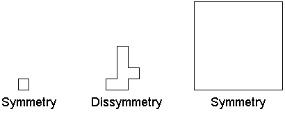
It is interesting to note that the basic element of a Cornucopia-type puzzle is symmetrical - a square, and the overall assembly is also symmetrical - likewise a square. A dissymmetry occurs between these two extremes in the permutated shape of the puzzle pieces. Thus, the order - symmetry - dissymmetry - symmetry represents in itself another, more abstract sort of symmetry (Fig. 43a).
Fig. 43a
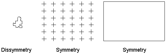
A typical die-cut jigsaw puzzle is an example of a different order of symmetry which is itself non-symmetrical (Fig. 43b).
Fig. 43b
A third order of symmetry would be represented by bathroom tiles on a typical floor (Fig. 43c).
Fig. 43c
Can you discover other orders of symmetry? This term, and in fact the whole concept of order of symmetry, was developed just as a curiosity as this chapter was being cut and pasted for at least the tenth time. This might be an interesting subject of study itself. Practically all puzzles described in this book are inherently of the symmetrical order: symmetry - dissymmetry - symmetry. The intriguing symmetries of the polyhedral shapes are often what attract the attention of the viewing public, much to the chagrin of the designer for all of the creative work lies hidden within and is so often overlooked.
Traditionally, artistic endeavors from music to poetry to oil paintings have nearly always been framed in symmetry of some sort or at least were until this century. Yet symmetry is a hopelessly sterile artistic medium within which to actually work. All creativity involves a judicious departure from symmetry inside this symmetrical framework.
Shown in Fig. 44 are all the ways that hexagonal blocks can be joined, up to size-four. (Incidentally, should the curious reader wish construct a set of hexagon pieces of size-five, one tedious but sure way to do this is to add an extra block to all of the size-four pieces in every possible position and then throw out the duplicates. You should end up with 22 pieces.)
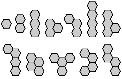
Fig. 44
Table 4
The most obvious problem shapes to construct with such pieces are hexagonal clusters. These are shown in Fig. 45 in increasing size.
Fig. 45
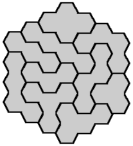
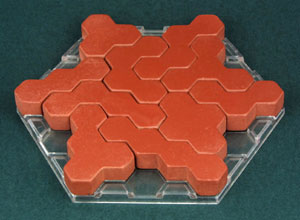
Thus, a set of the three size-three pieces plus the seven size-four pieces just happens to construct the 37-block hexagonal cluster (Fig. 46a). It also constructs a snowflake-shaped figure (Fig. 46b) plus many other geometrical and animated shapes. Beeler found by computer analysis that the hexagonal cluster has 12,290 solutions, and the snowflake pattern (from which a commercial version of this puzzle derived its name) has 167 solutions. The Snowflake Puzzle in Fig. 46c was cast from Hydrastone by Stewart.
Fig. 46c
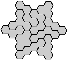
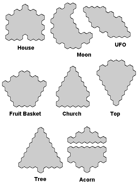
One of the special charms of this set of pieces is that it lends itself so well to creating geometrical, artistic, and animated puzzle problems. Just a few examples taken from the 10-page instruction booklet that came with the Snowflake Puzzle are shown in Fig. 47. The others are left for the reader to rediscover or improve upon. By the way, this is but one more example of a recreation in which young children excel. Many of the design patterns in the Snowflake Puzzle booklet were created by children under ten years of age.